Continuous glucose monitoring (CGM) generates a rich time‑series of glucose values, but extracting clinically meaningful information from these data is not always straightforward. Traditional summary metrics—mean glucose, standard deviation, time in range—offer a useful overview, yet they may miss subtle patterns in how glucose fluctuates. Two recent concepts aim to capture deeper aspects of glucose homeostasis: glucotype and glucodensity. Both move beyond simple averages to describe the distribution and temporal structure of glucose readings, opening new possibilities for patient characterization, risk stratification, and personalized management.
In this chapter we introduce these two concepts, explain how they are calculated, and illustrate their potential applications. No programming code is shown; instead we focus on the underlying ideas and how they can be used in clinical or research settings.
A glucotype is a categorical classification of a person’s glycemic variability derived from spectral clustering of CGM time series data (Hall et al. 2018). Instead of simply reporting a single number (like the coefficient of variation), the glucotype approach groups the data into three distinct patterns of glucose fluctuation:
Low variability – stable glucose levels with few abrupt changes.
Moderate variability – occasional fluctuations, but no extreme swings.
Severe variability – frequent and large glucose excursions.
This classification was originally developed using data from 57 non‑diabetic individuals, but it has since been applied to populations with diabetes as well.
7.2.2 How is a Glucotype Calculated?
The calculation involves three main steps:
Data segmentation – The CGM record is divided into overlapping windows of 2.5 hours each.
Spectral clustering – Each window is assigned to one of the three variability groups based on its spectral signature (i.e., the frequency components of the glucose signal).
Patient classification – For each individual, the proportion of time spent in each of the three groups is computed. The person is assigned to the group in which they spent the majority of the monitoring period.
7.2.3 Practical Tools for Glucotype Analysis
7.2.3.1 Single‑patient interactive web application
The authors of the original study provide a free interactive Shiny application that allows you to upload a CGM file and obtain the glucotype classification:
The input file must be a .tsv (tab‑separated values) with two columns: GlucoseDisplayTime (date‑time) and GlucoseValue (mg/dL). The application returns a visual summary of the glucose trace with color‑coded segments indicating the variability category for each 2.5‑hour window, as well as the final glucotype assignment.
Take the generated file [case1.tsv] and upload it here: Check my patient glucotype. Just Browse the file and click Classify glucotype.
This patient has: moderate glucotype. [32% is in low, 48% in moderate, and 20% in severe].
7.2.3.2 Bulk processing for multiple patients
For larger studies, the authors have released an R package (or set of scripts) on GitHub: abreschi/shinySpecClust. Using the provided functions (classify.R) and pre‑trained model parameters, you can automatically classify hundreds of subjects in a single run. (not covered yet in the present materials).
7.3 Glucodensity: A Distributional View of Glucose
7.3.1 What is Glucodensity?
Glucodensity is a novel way of representing CGM data by focusing on the probability distribution of glucose values rather than their chronological order (Matabuena et al. 2021). For each individual, a smooth density function is constructed that estimates how much time is spent at each glucose concentration. In other words, it answers the question: “What is the proportion of time my glucose was between 70 and 80 mg/dL, between 80 and 90, … and so on across the entire range?”
Formally, if \(Y(t)\) denotes the glucose level at time \(t\) over a monitoring period of length \(T\), the cumulative distribution function (CDF) is
and the glucodensity is its derivative \(f(x) = F'(x)\). Thus each patient is represented by a probability density curve (a functional object) that summarizes his or her glucose distribution.
7.3.2 Here it is! From Galicia to the World 🐙🐚🌊
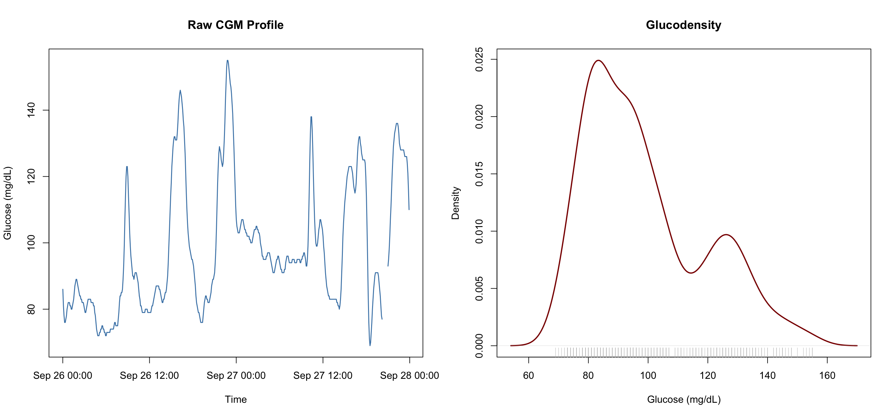
We provide a visualization with a dual perspective on glycemic control by combining glucodensity and a temporal trace. The relationship between these two plots allows researchers to move beyond simple averages to understand both the timing and the frequency of glucose levels.
Raw CGM Profile (Left) – The left panel shows the longitudinal timeline of glucose values over a two‑day period (September 26–28). The jagged peaks indicate individual “excursions,” while the valleys show the recovery phases.
Glucodensity (Right) – The right panel is the glucodensity that summarizes the entire CGM profile. It represents the time‑in‑state, showing exactly how much of the total recording period was spent at specific glucose concentrations.
# Load data (assuming the file contains columns: id, hora, glucemia)df <-read.csv("Colas/case 1.csv", header =TRUE)[, -1] # drop first column (index)# Convert time column to POSIXct (if not already)df$time <-as.POSIXct(df$hora, format ="%Y-%m-%d %H:%M:%S")# Side-by-side plotspar(mfrow =c(1, 2))# Left: raw CGM traceplot(df$time, df$glucemia, type ="l", col ="steelblue", lwd =1.5,xlab ="Time", ylab ="Glucose (mg/dL)",main ="Raw CGM Profile")# Right: glucodensity (kernel density estimate)dens <-density(df$glucemia, na.rm =TRUE)plot(dens, main ="Glucodensity",xlab ="Glucose (mg/dL)", ylab ="Density",col ="darkred", lwd =2)rug(df$glucemia, col ="gray")
Feature
Interpretation
Primary peak (~85 mg/dL)
The most frequent glucose concentration; reflects the subject’s stable “baseline” or fasting state.
Secondary peak (~130 mg/dL)
A “hump” indicating a significant amount of time spent at a higher level, likely corresponding to recurring post‑meal peaks seen in the raw profile.
Tail (beyond 150 mg/dL)
The thinning line to the right shows that while the patient reaches high levels, they spend very little total time in that extreme hyperglycemic range.
Together, these plots provide a complete metabolic picture. The raw CGM profile tracks the when (the sequence of events), while the glucodensity summarizes the how long (the overall exposure). For a clinician, the “bimodal” shape of the density plot—having two distinct peaks—clearly identifies a patient who oscillates between a healthy baseline and a consistent post‑meal elevation.
7.3.3 Why is Glucodensity Useful?
Richer information – It captures the entire distribution, not just a few summary statistics. Two patients with identical mean glucose and time in range can have very different glucodensities if one has a narrow peak centered at 120 mg/dL and the other has a wide, flat distribution.
Natural generalization of time in range – Time‑in‑range metrics are essentially the integral of the glucodensity over pre‑defined intervals. Glucodensity allows you to look at any interval, no matter how narrow, and to visualize the shape of the glucose distribution.
Improved clinical sensitivity – In the original validation (Matabuena et al. 2021), the authors showed that glucodensities could predict HbA1c, HOMA‑IR, and glycemic variability indices (CONGA, MAGE, MODD) with substantially higher accuracy than time‑in‑range metrics. Moreover, the reverse was not true: the standard biomarkers could not reconstruct the glucodensity precisely, indicating that the density representation contains information not captured by traditional measures.
7.3.4 The biosensors.usc Package
The methods developed for glucodensity analysis are implemented in the biosensors.usc R package, available on CRAN. The main functions include:
load_data() – Reads CGM data and prepares it for analysis.
hypothesis_testing() – Performs comparisons between groups, returning functional means, variances, and p‑values.
NOTE: we are testing all recorded glucose values not just the value of an index.
clustering() – Applies Wasserstein‑based clustering to identify patient subgroups.
Other techniques include: regression, ridge regression, missing data imputation, and more to come […]
For further details on the development of glucodensity and its applications in diabetes research, follow the work of Marcos Matabuena, whose contributions include the introduction of glucodensity as a functional representation of CGM data, uncertainty quantification in metric spaces, and advanced statistical methods for wearable devices. In that webpage scroll down a bit and check: Research in pictures.
7.3.5 Potential Clinical Applications
Glucodensity opens several avenues for improving diabetes care and research:
Personalized phenotyping – Identifying individuals with unusually shaped distributions (e.g., a bimodal pattern indicating alternating hypo‑ and hyperglycemia) may help tailor therapy.
Predicting outcomes – Because glucodensity captures long‑term glucose exposure more accurately than simple averages, it may better predict microvascular complications or response to treatment.
Monitoring interventions – The effect of a new diet, exercise program, or medication could be evaluated by how it changes the shape of the glucodensity curve, not just the mean glucose or time in range.
7.4 A biosensors.usc Data Analysis Example
In this section we walk through its main functionalities, illustrating how to go from raw CGM data to advanced statistical analyses.
7.4.1 Loading and Preparing Data
The first step is to prepare the CGM data in a format the package can handle. Typically, you need two files:
A glucose data file containing at least three columns: subject identifier (id), time stamp (time), and glucose reading (value). [similar to our colas_long.csv, just changing colnames, and we are there].
An optional clinical variables file with subject identifiers and any covariates (age, sex, BMI, diabetes status, etc.).
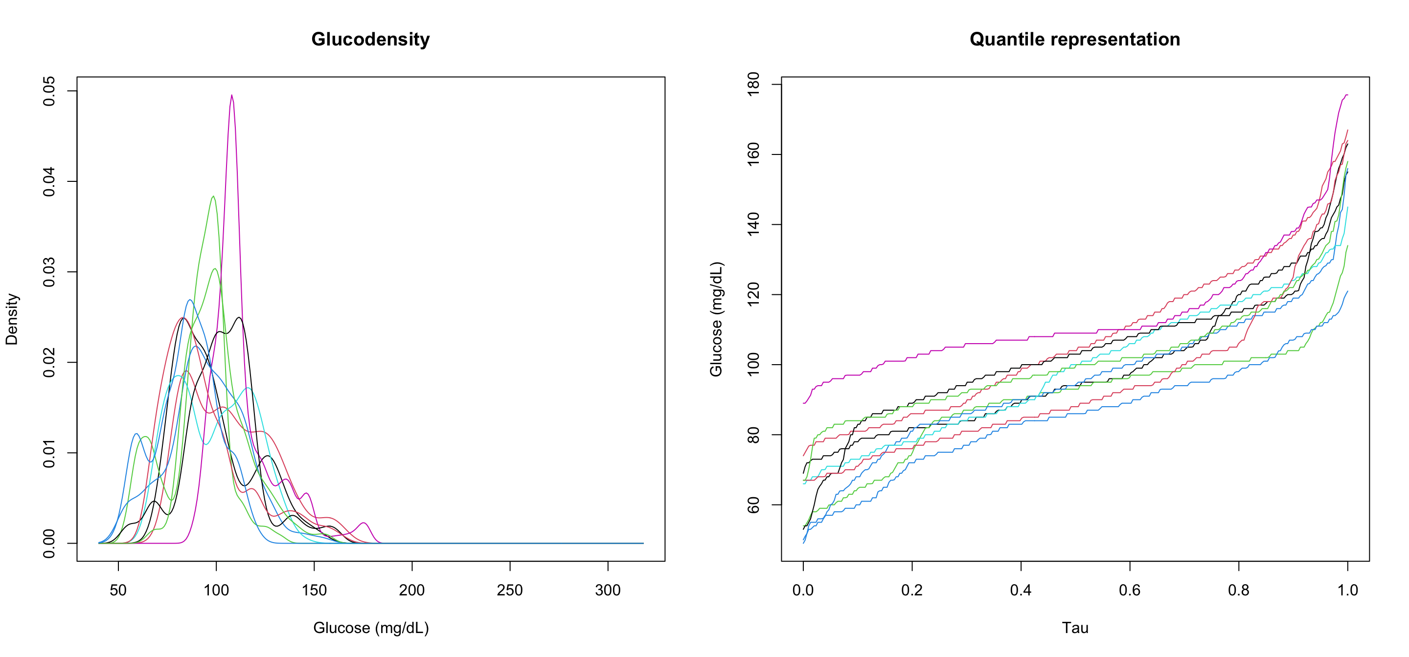
The load_data() function reads these files and constructs the necessary objects: for each subject it estimates the glucodensity (a probability density function of glucose values) and its quantile representation. Internally it uses kernel density estimation with a bandwidth selected to preserve the shape of the distribution.
library(biosensors.usc)# Read glucose data (adjust column names as needed)glucose <-read.csv("Colas_clinical/colas_long.csv")names(glucose)[names(glucose) =="gl"] <-"value"glucose$time <-as.POSIXct(glucose$time, format ="%Y-%m-%d %H:%M:%S")# Save temporary file for load_datawrite.csv(glucose, "biosensors/temp_glucose.csv", row.names =FALSE)# Load into biosensors.uscobj <-load_data("biosensors/temp_glucose.csv")# Plot first 10 subjectspar(mfrow =c(1, 2))plot(obj$densities[1:10, ], xlab ="Glucose (mg/dL)", ylab ="Density",main ="Glucodensity")plot(obj$quantiles[1:10, ], xlab ="Tau", ylab ="Glucose (mg/dL)",main ="Quantile representation")
7.4.2 A Test Comparison Between Two Groups
We compare the glucodensities of subjects with and without type 2 diabetes using the hypothesis_testing() function from biosensors.usc. Two complementary tests are performed:
Energy distance test – detects any overall difference in the distribution (location, scale, shape).
ANOVA‑type test – specifically tests for a difference in the Wasserstein mean.
# Read dataglucose <-read.csv("Colas_clinical/colas_long.csv")clin <-read.table("Colas_clinical/clinical_data.txt",header=T)# Prepare glucose data: rename "gl" to "value" and ensure time is POSIXctnames(glucose)[names(glucose) =="gl"] <-"value"glucose$time <-as.POSIXct(glucose$time, format ="%Y-%m-%d %H:%M:%S")# Subset IDs by diabetes statusid_nodm <- clin$id[!clin$T2DM]id_dm <- clin$id[clin$T2DM]# Create glucose data for each groupno_dm <- glucose[glucose$id %in% id_nodm, ]dm <- glucose[glucose$id %in% id_dm, ]# Corresponding clinical datavars_nodm <- clin[clin$id %in% id_nodm, ]vars_dm <- clin[clin$id %in% id_dm, ]# Write temporary fileswrite.csv(no_dm, "biosensors/no_dm.csv", row.names =FALSE)write.csv(vars_nodm, "biosensors/vars_nodm.csv", row.names =FALSE)write.csv(dm, "biosensors/dm.csv", row.names =FALSE)write.csv(vars_dm, "biosensors/vars_dm.csv", row.names =FALSE)# Load into biosensors.uscdata_nodm <-load_data(filename_fdata ="biosensors/no_dm.csv", filename_variables ="biosensors/vars_nodm.csv")data_dm <-load_data(filename_fdata ="biosensors/dm.csv", filename_variables ="biosensors/vars_dm.csv")# Hypothesis testhtest <-hypothesis_testing(data_nodm, data_dm)
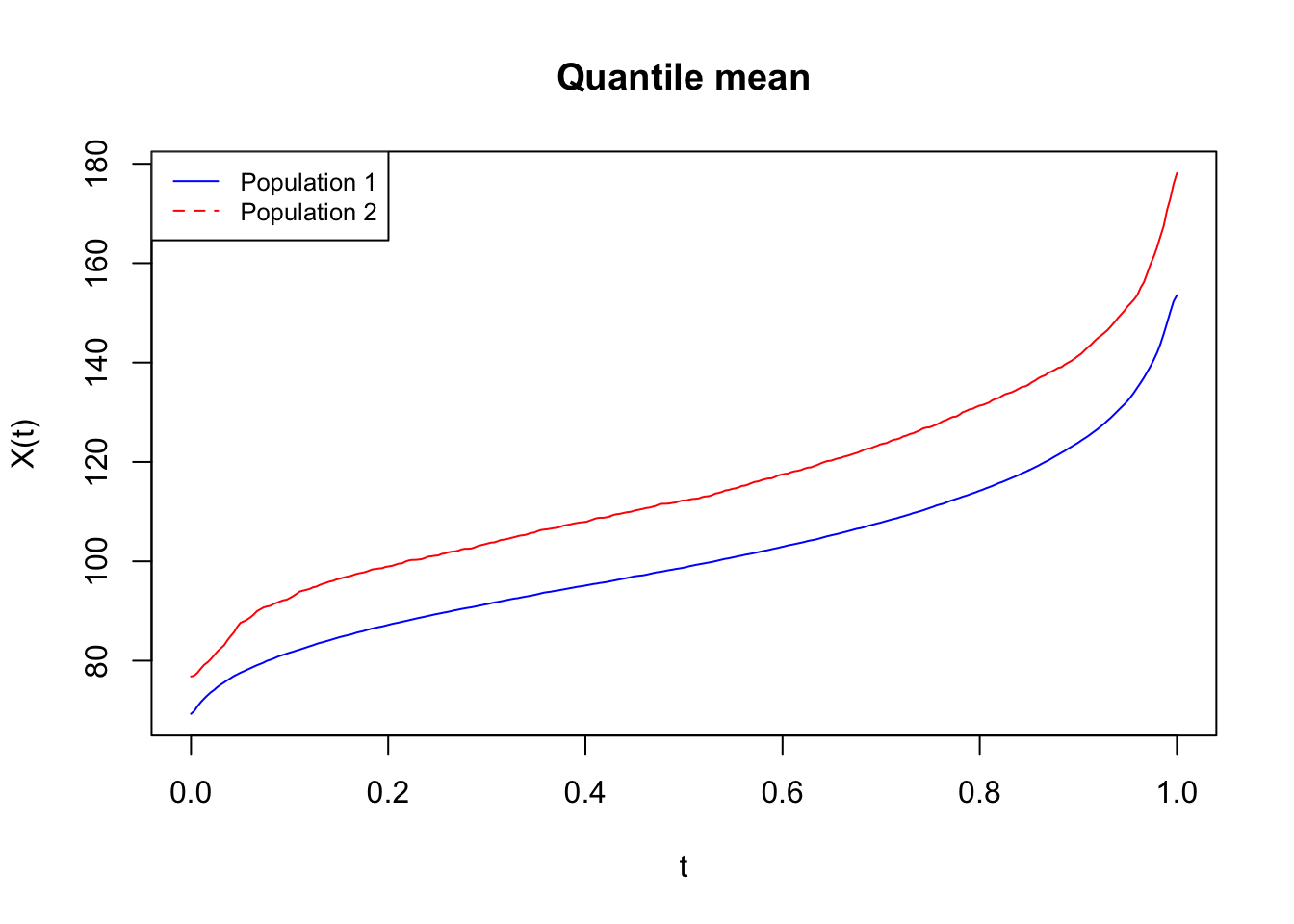
The quantile curves (top plot) show the distribution of glucose values over the entire monitoring period. The blue line (individuals who remained free of diabetes) stays lower and flatter—this is the signature of a healthy, resilient glucose control system. The red line (those who went on to develop diabetes) is shifted upward. Even before they were diagnosed, their glucose levels already tended to run higher, and their curves show a wider range, indicating early instability.
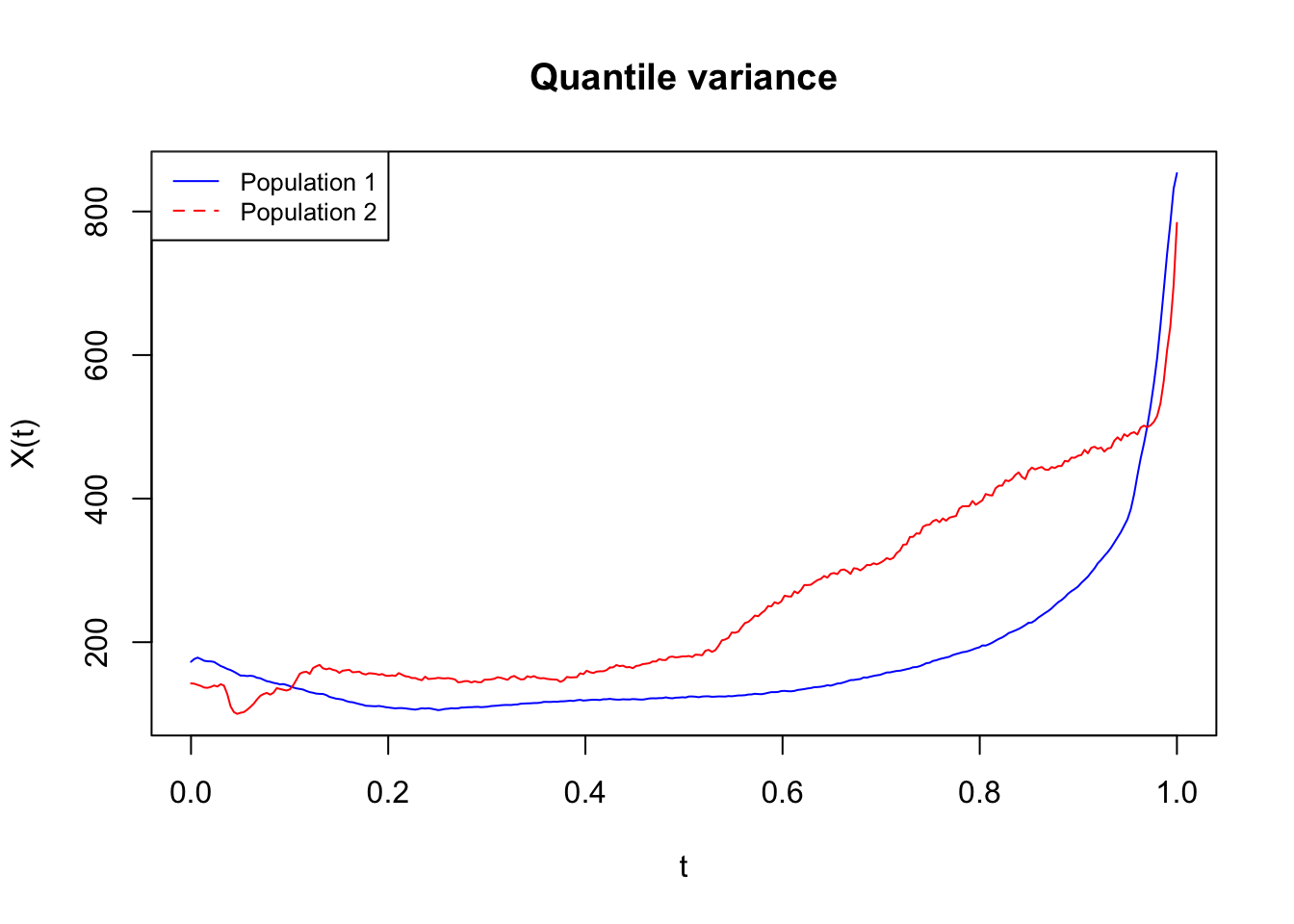
I will not explain the bottom plot here as I do not have a clear intuition of whats going on yet [still, it looks cool! 😎]
The p‑values confirm the importance of looking beyond simple averages:
Energy distance p‑value = 0 → There is a clear, statistically significant difference in the entire pattern of glucose between the two groups. Their metabolic “fingerprints” are fundamentally different.
ANOVA‑type p‑value = 0.25 → If we only looked at a simple average glucose, we might miss this difference.
This is why continuous glucose monitoring (CGM) is so powerful: it captures the shape and swings of glucose that appear years before clinical diagnosis.
Clinical takeaway
Early signals matter: People who will develop diabetes already show a higher baseline glucose and greater variability, even when their fasting glucose or HbA1c is still in the “normal” range.
Variability as a risk marker: The wider spread and second hump in the density plot highlight that unstable glucose patterns are an early harbinger of diabetes, not just a consequence of established disease.
Monitoring matters: For nursing practice, this reinforces that looking at a single glucose value is not enough. Understanding the patient’s typical range and swings can help identify those at risk and guide preventive interventions earlier.
7.5 Comparison of Glucotype and Glucodensity
While both concepts aim to extract richer information from CGM data, they take different approaches:
Feature
Glucotype
Glucodensity
Focus
Temporal patterns of variability (clusters of 2.5‑h windows)
Distribution of glucose values over the whole monitoring period
Output
Categorical (low / moderate / severe variability)
A continuous probability density function (functional data)
Use case
Quick classification of glycemic stability
In‑depth analysis of glucose distribution, hypothesis testing, clustering
Tools
Shiny app, GitHub scripts
biosensors.usc R package
Both methods complement traditional metrics. Glucotype is especially useful for a fast, clinically intuitive categorization, while glucodensity provides a more detailed statistical framework for research and advanced clinical decision support [from which a clinically intuitive categorization is also possible].
7.6 Conclusion
The advent of CGM has generated a wealth of data, but extracting its full value requires moving beyond simple summaries. Glucotype and glucodensity represent two innovative ways to characterize glucose homeostasis: one focuses on the temporal structure of variability, the other on the distributional shape. Both have demonstrated superior sensitivity compared to conventional metrics and hold promise for improving risk prediction, patient stratification, and personalized care (Shao et al. 2026)(Matabuena et al. 2025).
As these tools become more widely available—through open‑source software and user‑friendly web applications—they will likely become part of the standard toolbox for clinicians and researchers working with CGM data.
Hall, Heather, Dalia Perelman, Alessandra Breschi, Patricia Limcaoco, Ryan Kellogg, Tracey McLaughlin, and Michael Snyder. 2018. “Glucotypes Reveal New Patterns of Glucose Dysregulation.”PLoS Biology 16 (7): e2005143. https://doi.org/10.1371/journal.pbio.2005143.
Matabuena, Marcos, Rahul Ghosal, Javier Enrique Aguilar, Ayya Keshet, Robert Wagner, Carmen Fernández Merino, Juan Sánchez Castro, Vadim Zipunnikov, Jukka-Pekka Onnela, and Francisco Gude. 2025. “Glucodensity Functional Profiles Outperform Traditional Continuous Glucose Monitoring Metrics.”Scientific Reports 15 (1): 33662.
Matabuena, Marcos, Alexander Petersen, Juan C. Vidal, and Francisco Gude. 2021. “Glucodensities: A New Representation of Glucose Profiles Using Distributional Data Analysis.”Statistical Methods in Medical Research 30 (6): 1445–64. https://doi.org/10.1177/0962280221998064.
Shao, Mandy M, Agatha F Scheideman, David C Klonoff, Francisco Gude, and Marcos Matabuena. 2026. “Glucodensity-Based Models Outperform Time in Range and Glycemia Risk Index in Prediction Models.”Journal of Diabetes Science and Technology, 19322968261421954.